Drains, sprinklers, and sidewalk edges: behind the development of Greenzie's first ML Model
Originally published on the Greenzie blog, this covers a project I led to deploy an image segmentation model on autonomous commercial lawnmowers.
A never-ending problem for mobile robotics is funneling a petabyte-dense visual world into just enough megabytes to help the robot act correctly in realtime. One example of this for autonomous mowing: identifying and navigating around small obstacles like sprinklers that could be damaged (or damage the mower).
Our team at Greenzie decided that the best way to identify small obstacles was to develop a custom image segmentation model. Here’s a look at how we’re developing and deploying this model to our fleet of autonomous lawnmowers.
The problem
Greenzie autonomous lawnmowers use a set of stereo cameras to generate a 3D point cloud of its surroundings. We group points into clusters to identify obstacles that the robot needs to avoid. However, it’s not easy identifying the classification of an object from a point cloud. For example, below is a side-by-side display of the depth cloud output and the image display from a stereo camera (source):
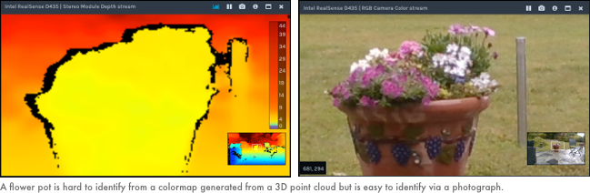
It’s not possible to identify the object in the depth display as a flower. It’s easy using the photo. In fact, off-the-shelf computer vision models can identify these as flowers. A point cloud cannot.
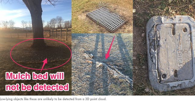
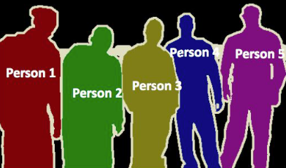
So, if Greenzie can already navigate around obstacles, why do we need an additional layer in our perception stack? Maybe we’re just trying to add “AI-powered™” stickers to our robots? Well, many obstacles are aligned close enough to the ground plane that they can be difficult to identify from a point cloud. Some of these objects could be damaged if the mower were to travel over them with the blades on. Some could damage the mower. For example, the objects in the image below can be difficult to detect in a 3D point cloud:
Adding the ability for our robots to sense additional objects via an image segmentation model gives us two big wins:
- Avoid an additional class of collision events (impacts with small obstacles).
- Increase the ROI our customers experience by increasing our robot’s confidence to navigate near small obstacles, reducing manual cleanup work.
Deciding on the ML model type
In the introduction, I quickly jumped to our decision to create an image segmentation model. Let’s take a quick look at the 3 types of models we considered.
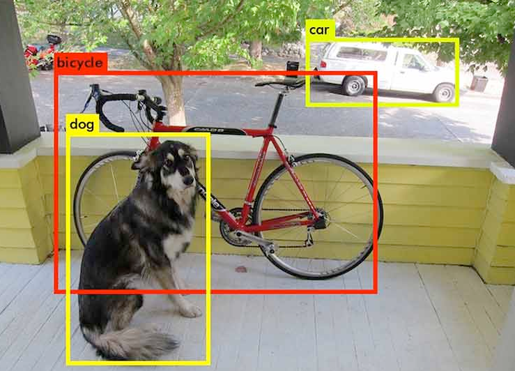
1. Object detection
This approach generates a bounding box around identified objects. For example, we could train a model to identify obstacles and their classification much like how this model identifies dogs, bikes, and other objects:
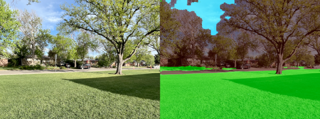
2. Image segmentation
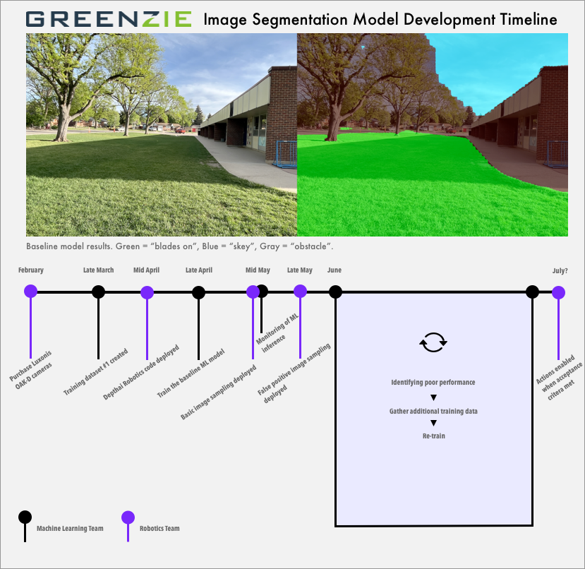
This classifies the category of items at the pixel-level rather than using a bounding box. For example, here’s an image segmentation result showing the sky, grass, and not-grass:
3. Instance segmentation
This combines both of the above approaches, allowing the model to identify individual instances of items in an image at the pixel-level. For example, you could count the number of mulch beds.
Why did we go with image segmentation?
We would like precise contours of “blades on”, “obstacle”, and “sky” regions (rules out object detection). We don’t need to identify individual instances of objects that an instance segmentation model offers.
With the problem defined and the ML model type chosen, development was ready to begin.
Step 1: pick the deployment platform (Luxonis OAK-D camera)
Our current platform uses a set of Intel Realsense cameras to capture images and depth data. However, we were concerned about the resource usage of running ML models on the host. We just happened to have a convenient mounting location for a Luxonis OAK-D camera. We can deploy the model to the OAK-D, keeping resources open on the computer for our other robotic work.
Step 2: create a training dataset for the image segmentation model
We used an iPhone to photograph areas similar to what our robotic workers mow. This included extensive photos of obstacles that could be within the mowing map and not seen by our depth cloud obstacle logic. These photos were sent to an image annotation service.
There’s no getting around it: assembling and reviewing annotation results is a tedious process. I felt more like a bookkeeper than a developer. That said, it was a valuable introspective process that showed where our annotation guidance was not clear. For example:
- Do you label every visible piece of grass visible behind a chainlink fence as “blades on”? Or the entire fence itself as an obstacle?
- Do you label grass visible behind a set of tree branches as “blades on”?
- What about small dirt patches within a grass area?
Let’s look at an example of annotation instructions gone wrong. Our initial instructions to the annotation service asked them to classify images into three classes: sky, obstacles, and grass. Look at some of these initial model results in photos from the field:
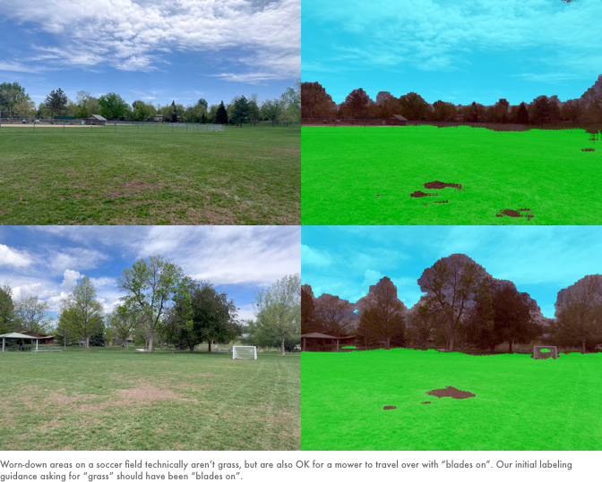
In the above model inference results, the overlays show how worn-down, high-traffic areas of a soccer field are classified as “not grass”. This is technically correct, but would be annoying when operating the mower. The mower will stop and/or navigate around these areas. It’s OK to have blades on over these areas.
Based on this experience, we updated our instructions changing the “grass” classification to “blades on”. The classification “blades on” now includes dirt patches.
Step 3: deploy the DepthAI Robotics Code
Greenzie’s robotic lawnmowers use the Robot Operating System (ROS). We worked with the Luxonis team to integrate the sensor data from the OAK-D camera into our system via their ROS DepthAI package. To start, we deployed an off-the shelf model (TinyYOLO4) to verify the end-to-end functionality.
Step 4: training a baseline image segmentation model
We again worked with Luxonis to develop the image segmentation model. Their team selected images for the training dataset, sent the images off for annotation, and trained the first several versions of the model. Our team focused on building a reproducible training environment on AWS Deep Learning Images once Luxonis completed a couple ad-hoc training sessions.
Step 5: basic image sampling from the field
Our training dataset was collected via an iPhone, not image data from robots in the field. This is convenient (and there isn’t a lot of mowing in the winter), but it was a risk. It’s not the same environment.
We developed sampling logic that saves an image from the OAK-D camera once-per minute. These are sent to the cloud where we can perform later analysis of the results.
Step 6: monitoring ML inference results
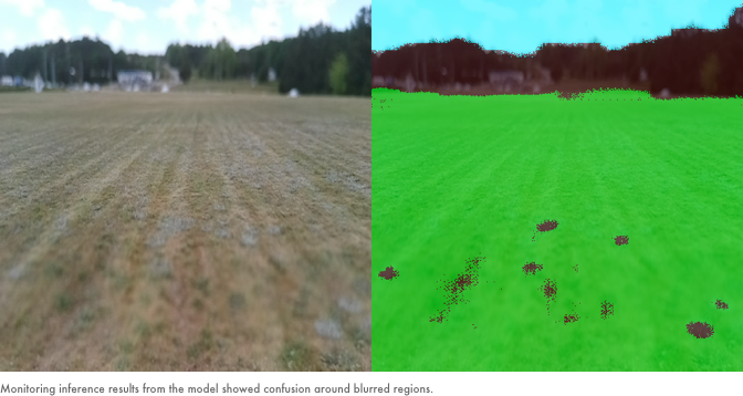
With image sampling in place, we developed a pipeline to transfer the images to S3 and generate side-by-side comparisons of the robot image with the model inference results. This identifies areas where the model was confused. For example, notice that the model struggled with identifying grass in blurred regions:
Now that mowing season is in-full swing, the size of our monitoring dataset will increase by several orders of magnitude and comes from the source-of-truth: the production sensors, running real customer mowing jobs.
Step 7: the refinement cycle
With monitoring of production ML inference in place, we’ll move faster refining the model to meet the criteria for acting on the results. This will help us address the rough edges faster. We’ll be cycling through previous steps: evaluating real-world inference results, augmenting our training dataset with new scenarios, and retraining the model.
Step 8: collecting data on false positives and false negatives
Once per-minute sampling is great, but it comes at a low signal to noise ratio. The vast majority of the time there are no obstacles in the mowing area. To collect more fine-grained data, we implemented the following in our ROS codebase:
- Collect false positives - save an image when the robot travels over an area that the ML model believes is an obstacle.
- Collect false negatives - save an image when our depth-cloud logic identifies an obstacle but the ML model does not.
We’re at the beginning of this more nuanced approach to gathering data.
Step 9: setting a threshold for enabling the model
It’s important to define “good enough” model performance or the cycle of retraining would never end. The model won’t be perfect at identifying small obstacles, but neither is a human operator. We’ve established the following criteria prior to enable the robot to act on the model inference results:
- Fewer than 1 false positive per-hour of autonomous mowing - a false positive results in frustrating scenarios for operators: missed patches if the mower navigates around an obstacle or a full-stop if the mower is unable to find a path around an obstacle.
- 70% true positive rate - wait a minute…this means the robot will collide with 3 of every 10 obstacles! How is that acceptable? Well, we’re phasing in the robot’s actions. Initially, the ML model results only augment what we’re already doing via the point cloud-based obstacle logic. Many of these low-lying objects won’t be seen by the point cloud logic, so this means we’re significantly reducing collisions at this threshold.
Once these are met, we’ll set new metrics (or just update these thresholds) for enabling the mower to interact more precisely around the boundary areas between “blades on” and “obstacles” (such as mowing more precisely around a mulch bed).
What’s next?
We’re beginning the final push: that last 10% of refinement that will take a bit of time to fully enable in production. These are possible areas we could explore next:
- A more efficient model refinement flow - collecting images, noting poor classification, sending off new images for labeling, and re-training is a tedious process. We’ll look at ways to make this more enjoyable.
- Exploring new areas - we are impressed with how well the model performed with our baseline training images. This gives us a lot of hope for other perception-related problems that could be solved with ML.